
How training scales: loss, compute and tokens · Technical gear
You will be able to: state the next-token cross-entropy objective and what a lower validation loss licenses you to claim about a downstream Big Widget task; use a published scaling study's fitted allocation, under its stated conditions, to decide whether a baseline should move towards more parameters or more tokens at fixed compute, and name a condition that breaks the transfer; and describe byte-pair encoding precisely enough to predict where it fragments text, and quantify the resulting cost, latency and context gaps.
Facts about particular models, tokenizers and studies are dated in the text. This module is as of November 2026. Big Widget Company and its plans are made up for teaching. Read the primary papers in sources.yml for full methods; Kaplan et al. (2020) is a preprint, the others are peer-reviewed. Anything we did not verify is marked "not checked".
Scope. Everything below concerns autoregressive, subword-tokenized text models of the kind the cited studies trained. We make no claim that every language model is autoregressive or uses this objective.
1. The objective
An autoregressive language model defines
p_\theta(x_1,\dots,x_T) = \prod_{t=1}^{T} p_\theta(x_t \mid x_{<t}),over token sequences, and pre-training minimises the average negative log-likelihood of the next token,
\mathcal{L}(\theta) = -\frac{1}{T}\sum_{t=1}^{T} \log p_\theta(x_t \mid x_{<t}).GPT-3 is "an autoregressive language model with 175 billion parameters".1 Kaplan et al. "optimize the autoregressive log-likelihood (i.e. cross-entropy loss) averaged over a 1024-token context", report it in nats, and record it on a held-out WebText2 test set and on other text distributions.2 The Transformer's decoder is likewise "auto-regressive" at each step, "consuming the previously generated symbols as additional input when generating the next", with a softmax producing "predicted next-token probabilities".3 The Transformer paper is architecture background: it was built for translation (and also tested on English constituency parsing), not as a pre-trained language model.3 Hoffmann et al. describe the large language models of 2022 as "large autoregressive transformers", citing it.4
Per position, the loss is $-\log p_\theta(x_t \mid x_{<t})$: the surprisal of the token that occurred. Its exponential, $\exp(\mathcal{L})$, is the perplexity. Two properties of the definition matter for what follows:
- It is distribution-bound. $\mathcal{L}$ is an expectation over a particular text distribution. Kaplan et al. found that "transfer to a different distribution incurs a constant penalty but otherwise improves roughly in line with performance on the training set".2
- It is uniform in weight, not in contribution. "Our current objective weights every token equally and lacks a notion of what is most important to predict and what is less important" (GPT-3, section 5).1 Every term enters with the same coefficient $1/T$; the terms themselves differ. By our arithmetic, a token predicted with probability 0.9 contributes about 0.105 nats of surprisal and one predicted with probability 0.001 about 6.91 nats. So a mispredicted critical token (a torque value, a part number, a defect class) can carry a large term. What the objective lacks is any task-importance weight: a change of $\Delta$ nats at one position moves $\mathcal{L}$ by only $\Delta/T$, so over a 1,024-token context a task-deciding error of a few nats shifts the average by under 0.01 nats (our arithmetic). The aggregate can barely move while the task answer flips.
2. What a validation-loss difference licenses
Evidence for. GPT-3's Figure 3.1 shows validation cross-entropy loss following "a power-law trend with the amount of compute used for training". The authors address the worry that "these improvements in cross-entropy loss come only from modeling spurious details of our training corpus", and report that they "lead to consistent performance gains across a broad spectrum of natural language tasks".1 Aggregate loss is a useful, low-variance training signal.
Limits.
- The link is not uniform across tasks: GPT-3 found "relatively smooth increases in many (though not all) downstream tasks", and some "on which few-shot performance struggles, even at the scale of GPT-3", naming natural-language inference (ANLI) among them.1
- Kaplan et al.'s discussion leaves it open: "it will be important to investigate whether continued improvement on the loss translates into improvement on relevant language tasks".2
- Contamination biases loss downwards. Reporting Chinchilla's language-modelling results, Hoffmann et al. caution that with four times more training data than Gopher, "train/test set leakage may artificially enhance the results".4 In their scaling analysis they use smoothed training loss as an estimate of test loss, justified, the authors say, because every run uses fewer training tokens than the corpus holds (the "infinite data regime"; section 1, footnote 2).4 That is a statement about corpus size, not a guarantee that no subset is ever sampled twice (see section 5).
At Big Widget. Two checkpoints of an in-house model. Checkpoint A: lower validation loss on a held-out general-text split. Checkpoint B: higher task score on the plant's defect-report summaries, graded by engineers on a held-out set. The claims each number supports:
| Number | Claim it supports | Claim it does not support |
|---|---|---|
| A's lower validation loss | A assigns higher likelihood to held-out text from that split | A writes better defect summaries |
| B's higher task score | B's summaries were judged better on that test set by those graders | B is a better language model in general |
Ask "out of how many?" before either number: the size of the held-out split, the number of summaries graded and the number of graders. This made-up example does not give them; a real report must. For a release decision about defect summaries, the task score (with its interval; see 400.6) is the evidence. A loss difference can motivate which checkpoints to evaluate; it cannot replace the evaluation. The quality lead, not the metric, makes the release decision.
3. Scaling laws and the compute constraint
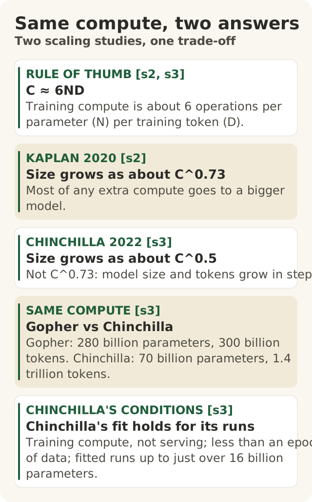
Figure data as text
Same compute, two answers
| Study or rule | What it shows |
|---|---|
| RULE OF THUMB [s2, s3] | C ≈ 6ND. Training compute is about 6 operations per parameter (N) per training token (D). |
| KAPLAN 2020 [s2] | Size grows as about C^0.73. Most of any extra compute goes to a bigger model. |
| CHINCHILLA 2022 [s3] | Size grows as about C^0.5. Not C^0.73: model size and tokens grow in step. |
| SAME COMPUTE [s3] | Gopher vs Chinchilla. Gopher: 280 billion parameters, 300 billion tokens. Chinchilla: 70 billion parameters, 1.4 trillion tokens. |
| CHINCHILLA'S CONDITIONS [s3] | Chinchilla's fit holds for its runs. Training compute, not serving; less than an epoch of data; fitted runs up to just over 16 billion parameters. |
Let $N$ be the number of non-embedding parameters, $D$ the number of training tokens and $C$ the training compute in FLOPs. Kaplan et al. estimate the non-embedding training compute as $C \approx 6N$ FLOPs per training token, so
C \approx 6ND,and Hoffmann et al. adopt the same approximation, "FLOPs(N,D) ≈ 6ND".24 Hoffmann et al.'s more detailed count (Appendix F) differs from $6ND$ by a ratio of 0.99 to 1.10 across their model sizes, and they "find the differences in FLOP calculation to be very small".4
Kaplan et al. report that "The loss scales as a power-law with model size, dataset size, and the amount of compute used for training".2 For compute-efficient training they find
N_{\text{opt}} \propto C^{0.73},with data requirements "growing very slowly as $D \sim C^{0.27}$", and conclude that "optimally compute-efficient training involves training very large models on a relatively modest amount of data and stopping significantly before convergence".2 They also state that the trends cannot hold indefinitely: "performance must flatten out eventually before reaching zero loss", and their scaling laws "must break down" at scales several orders of magnitude above those they documented (section 6.3).2
4. Compute-optimal allocation (Hoffmann et al. 2022)
Hoffmann et al. pose the problem as
N_{\text{opt}}(C),\, D_{\text{opt}}(C) = \arg\min_{N,D \,:\, \text{FLOPs}(N,D) = C} L(N,D),and estimate it three ways from over 400 runs between 70 million and just over 16 billion parameters.4 Fitting $N_{\text{opt}} \propto C^a$ and $D_{\text{opt}} \propto C^b$ (Table 2):4
| Approach | $a$ | $b$ |
|---|---|---|
| 1. Minimum over training curves | 0.50 | 0.50 |
| 2. IsoFLOP profiles | 0.49 | 0.51 |
| 3. Parametric loss fit | 0.46 | 0.54 |
| Kaplan et al. (2020), as listed | 0.73 | 0.27 |
Hence "the model size and the number of training tokens should be scaled equally": "for every doubling of model size the number of training tokens should also be doubled".4
The third approach fits
\hat{L}(N,D) = E + \frac{A}{N^{\alpha}} + \frac{B}{D^{\beta}},where $E$ is described as the entropy of natural text, the $A$ term the shortfall of a finite model and the $B$ term the shortfall of finite training.4 Appendix D.2 reports $E = 1.69$, $A = 406.4$, $B = 410.7$, with exponents 0.34 on $N$ and 0.28 on $D$.4 Minimising under $6ND = C$ gives (their equation 4)
N_{\text{opt}}(C) = G\left(\frac{C}{6}\right)^{a},\quad D_{\text{opt}}(C) = G^{-1}\left(\frac{C}{6}\right)^{b},\quad G = \left(\frac{\alpha A}{\beta B}\right)^{\frac{1}{\alpha+\beta}},\quad a = \frac{\beta}{\alpha+\beta},\ b = \frac{\alpha}{\alpha+\beta}.With the rounded exponents above, $a \approx 0.45$ and $b \approx 0.55$ by our arithmetic, against the fitted 0.46 and 0.54 in Table 2; the gap comes from rounding and is not checked further here.
The test at scale. Gopher: 280 billion parameters, 300 billion tokens. Chinchilla: 70 billion parameters, 1.4 trillion tokens, trained with the same compute budget, by the authors' account.4 The paper gives two figures for Gopher's budget. Table 3 uses $5.76 \times 10^{23}$ FLOPs (the Gopher paper's figure) as its "Gopher unit"; Appendix F says the paper's own, more accurate count gives $6.3 \times 10^{23}$.4 By $6ND$, our arithmetic gives about $5.0 \times 10^{23}$ FLOPs for Gopher and $5.9 \times 10^{23}$ for Chinchilla. These are rough approximations from rounded counts, not the detailed accounting; the same-compute comparison is the authors' claim, not something the rounded $N, D$ counts prove on their own. The ratio of tokens to parameters is about 1.1 for Gopher and 20 for Chinchilla (our arithmetic from the published counts). Chinchilla "uniformly and significantly" outperformed Gopher, GPT-3, Jurassic-1 and Megatron-Turing NLG on a large range of downstream evaluations.4
The 20 tokens per parameter is Chinchilla's own ratio at Gopher's budget, not a constant the paper prescribes for every budget; the paper gives the optimum as a function of $C$ (its Table 3) and reports curvature at high compute (section 5 and Appendix E).4
5. Deciding a reallocation, and when it does not transfer
Procedure. Given a baseline $(N_0, D_0)$ at budget $C_0 \approx 6N_0D_0$:
- Check the study's conditions (below) against your setting.
- If they hold, compare the baseline's tokens per parameter, $D_0/N_0$, with the study's optimum at a comparable budget. A baseline far below it is undertrained for its size.
- At fixed $C_0$, $N \cdot D$ is fixed, so moving towards the optimum means shrinking $N$ and growing $D$ by the same factor $k$: $(N_0/k,\ kD_0)$. A baseline far above the optimum would move the other way.
At Big Widget. The research team's first plan for a model trained on its service and engineering text has $D_0/N_0 \approx 1$, Gopher's regime. Under the study's assumptions, the reallocation is fewer parameters and more tokens at the same $C_0$. Then the conditions:
| Condition in the study | What it means for transfer |
|---|---|
| The objective minimises loss at a fixed training budget, $\text{FLOPs}(N,D) = C$.4 | Serving cost is not in the objective. The paper notes Chinchilla's "reduced model size reduces inference cost considerably".4 A model served millions of times a day makes inference cost part of the decision; the study's optimum does not account for it, so the training-optimal $(N, D)$ is not automatically the deployment-optimal one. |
| "the training runs for our analysis have all been trained on less than an epoch of data"; "future work may consider the multiple epoch regime".4 "Less than an epoch" means fewer training tokens than the corpus holds (footnote 2), not that nothing repeats: Chinchilla's 1.4T-token validation run took about 1.24 epochs of MassiveWeb and 3.40 of Wikipedia (Appendix A, Table A1).4 | Distinguish the scaling-analysis runs from the Chinchilla validation run, and total corpus size from repeated sampling of subsets. What the fits do not establish is many complete passes over a small corpus. If Big Widget's text is too small to reach $kD_0$ without that, the result is untested for that regime. The authors also suggest, speculatively, that "scaling to larger and larger datasets is only beneficial when the data is high-quality".4 |
| Fits up to just over 16B parameters; "we only have two comparable training runs at large scale (Chinchilla and Gopher)"; "some concavity" at high compute; "significant uncertainty extrapolating out many orders of magnitude".4 | A budget far outside the tested range is extrapolation. |
| The target is loss on the study's own data (MassiveText); Appendix C repeats the analysis on C4 and GitHub code, with similar exponents, for single-epoch training.4 | Loss is not the Big Widget task metric (section 2), and a domain corpus is another distribution. |
The two studies' exponents (0.73 and about 0.5) differ on the same question, which is itself evidence that a scaling law is a fitted result under conditions, not a law of nature.24 Big Widget's usable token count is not known yet; the team measures it before the research lead, who owns the plan, commits the budget.
6. Subword tokenization: byte-pair encoding
The model consumes integer token ids from a fixed vocabulary; disparities between languages arise "at the tokenization stage, well before the language model sees any data at all".5 "Subword tokenization is currently the preferred approach for state of the art language models".5
Sennrich, Haddow and Birch (ACL 2016) adapted byte-pair encoding, a compression algorithm, to word segmentation, "encoding rare and unknown words as sequences of subword units".6 Section 3.2:
vocab  <- set of characters in the corpus (plus an end-of-word marker)
repeat M times:
    count every adjacent symbol pair in the corpus (weighted by word frequency)
    (x, y) <- the most frequent pair
    replace every occurrence of (x, y) with a new symbol xy; add xy to vocab
"The final symbol vocabulary size is equal to the size of the initial vocabulary, plus the number of merge operations", and the number of merges "is the only hyperparameter of the algorithm".6 "Frequent character n-grams (or whole words) are eventually merged into a single symbol", so frequent strings become single tokens and rare strings fragment.6 A token can therefore be a whole word, a word piece or a single character, depending on the learned merges.6 The Transformer's English-German experiments used byte-pair encoding with "a shared source-target vocabulary of about 37000 tokens".3 GPT-3 reuses GPT-2's byte-level BPE; its tokens average "∼0.7 words per token", so character-level tasks require "pulling apart" a token's substructure.1
Because merges are ranked by corpus frequency, the vocabulary encodes the training corpus. Petrov et al. (NeurIPS 2023) show GPT-2 has a dedicated token for "BuyableInstoreAndOnline" while the Bulgarian word "защо" ("why") needs 6 tokens for 4 letters, and note: "If one uses non-natural inputs, log files, or specialist forums, the tokenizer vocabulary would reflect this."5
7. Tokenization premiums and their costs
Petrov et al. define the premium for language $A$ relative to $B$ on a parallel sentence pair $(s_A, s_B)$ as
\text{premium}_{A|B} = \frac{|t(s_A)|}{|t(s_B)|},with parity when it is close to 1, and measure it on FLORES-200: the same 2,000 Wikipedia sentences human-translated into 200 languages.5 For the cl100k_base tokenizer used by ChatGPT and GPT-4 at the time of the paper (2023), the premium relative to English was about 1.6 for Italian, 2.6 for Bulgarian and 3 for Arabic, and up to 15 for Shan.5 Byte-level encodings are not neutral either: "over 4 times the difference in the encoding length for some language pairs".5
The premium bears on three operating quantities, under different assumptions. Keep them separate.5
- Input charge (an assumption about billing). "Commercial services charge users per token or Unicode character". Under per-token pricing at a common price per token, and for otherwise comparable requests, the input-token premium maps directly to an input-charge premium (section 5.1); users of some languages pay "at least 2.5 times more for the same task as users of English". Under per-character billing the token premium does not set the price, and output length and the provider's price schedule also enter a real bill. Per-character billing is not neutral either: the same content needs different character counts in different languages (section 5.1).5
- Context (arithmetic on a fixed budget). With a fixed context of $n_{\text{ctx}}$ tokens, the content that fits scales as $n_{\text{ctx}} / \text{premium}$; token-efficient languages can fit texts "more than an order of magnitude longer".
- Latency (an empirical measurement). Some languages "can require twice the time to process the same content as English". Section 5.2 reports processing time for one model, RoBERTa, growing roughly linearly with tokenization length rather than quadratically. That is one measurement, not a general law for a served model: batching, hardware, output length and serving stack all enter. Measure latency on the configuration you will deploy.
Quality effects are plausible but harder to attribute. GPT-3's English-to-Romanian translation was "a noticeable outlier", over 10 BLEU worse than prior unsupervised translation work; the authors write that this "could be a weakness due to reusing the byte-level BPE tokenizer of GPT-2 which was developed for an almost entirely English training dataset", a hypothesis, not a measured cause.1
Part numbers. A string such as BWX-40417-QR (a made-up Big Widget part number) is rare in public web text, so a BPE vocabulary learned from that text may, by the merge rule above, cover it with several tokens rather than one.6 We have not tokenized it, or any one-character variant of it, with any tokenizer: the split, the token count and how a single-character edit changes the token sequence are all not checked. Treat fragmentation as a conditional risk, not a measured property. To quantify it, tokenize the identifier with the deployed tokenizer and compare against an explicit baseline (for example, a one-token-per-identifier ideal), and tokenize near-miss variants too. Because the risk is wrong output rather than a known incapacity, test it as output: exact-match checks that identifiers survive a round trip through the model.
At Big Widget. The service team measures the premium of each supported language against English on its own parallel instructions, using the tokenizer of the model it will deploy. It confirms its provider's billing scheme and measures latency on its own serving configuration. The service lead sets per-language cost, latency and context budgets from those measurements. The team adds exact-match tests that part numbers survive a round trip through the model.
8. The three yeses for training and tokenizer decisions
A validation loss, a fitted exponent and a premium are evidence. None is a permission, and neither the model nor the metric makes a decision. Each decision below has a named owner at Big Widget, and each yes is scoped: one checkpoint, one $(N, D)$ plan or one set of languages and identifiers, for one use. The gate's answer is one of allow, constrain, hold or deny (go ahead, only this far, wait for a person, no).
| Movement | Gate (from the Foundation's lifecycle) | Application in this module |
|---|---|---|
| Get to Yes | Before the plan or release is approved | State the exact decision and the evidence that fits it: a held-out task score with its counts for a checkpoint release (quality lead), the study's conditions checked one by one for a $(N, D)$ plan (research lead), measured premiums, billing and latency for per-language limits (service lead). A typical constrain: allow the languages whose premiums and latency have been measured, hold the rest. |
| Stay at Yes | While the model runs | Track the task score, not only the loss, across checkpoints. Re-measure premiums when a language is added or the model or tokenizer changes. Keep the identifier exact-match tests in the running suite. |
| Recover to Yes | After an incident, on demand | If an identifier comes back altered: hold drafts that quote identifiers for human checking against the parts list, contain affected outputs, and have the service lead own the repair and notify anyone affected. Verify with a deterministic string comparison, not by asking the same model whether it copied correctly. A hold is containment, not recovery; claim recovery only when the exact-match suite passes again on the repaired configuration. |
Records and receipts. Test sets, scores, token counts and the decision log live in the team's own controlled work record. Defect reports, customer text and manuals are not pasted into anything shared beyond it. A signed receipt of a gate decision carries metadata (hashes, the decision, policy and key references), never prompts, outputs, payloads or personal data; it shows a decision was recorded, not that the evidence behind it was right. (This is a course rule; module 100.P covers the format.)
Unknowns. "I don't know yet" is a valid entry, for example for Big Widget's usable token count. Record it with the person who will measure it; the decision waits for its owner.
Words to know
autoregressive factorisation, cross-entropy, surprisal, perplexity, distribution shift, contamination, $C \approx 6ND$, compute-optimal frontier, IsoFLOP profile, parametric loss fit, epoch, inference cost, byte-pair encoding, merge operation, tokenizer parity, tokenization premium.
Further learning (optional, not sources)
Free university materials that go deeper. Pointers only; nothing in this module is copied from them, and we found no licence for any of them.
- Stanford University, CS336: Language Modeling from Scratch (Spring 2025): tokenizer and scaling-law assignments on the public archive; some files were not reachable when checked on 18 November 2026.
- Carnegie Mellon University, 11-711 Advanced Natural Language Processing (Spring 2025)
- University of Oxford, Deep Natural Language Processing (2017 lectures)