
Operating a model: monitoring, drift and rollback · Technical gear
As of 18 Nov 2026. Reviewed and published, version 1.0.0, part of How AI Works, the AiGovOps Foundation's planned free course. It is not a credential. Results are dated and hold for the settings their authors tested. No real operating incident is used: the worked example is a made-up record, labelled as such. Arithmetic marked "course arithmetic" is this course's own illustration, not a result from the sources. Unknowns are stated as unknown, with an owner.
You will be able to:
- extend a Level 300 hold card (holder, thresholds, stop) with versioned monitoring that detects input shift and performance decay under delayed labels, and state the paging threshold and how its false-page rate will be measured;
- write a release manifest that pins model, data, code and configuration under one release ID, gate and stage the rollout, and name who may stop it;
- identify entanglement, hidden feedback loops and undeclared consumers in a system diagram, and attach one control to each.
Big Widget Company, its people, systems and numbers are made up for teaching.
Fixture: the made-up release-and-monitoring record
Target: weekly order count $y_{d,w}$ for dealer $d$ in week $w$. The model $f$ emits a forecast $\hat y_{d,w}$. Labels are final at $w+6$ weeks. Consumers: parts planning (declared), pricing tool (declared), a finance warranty-reserve spreadsheet (undeclared; see section 3).
| Day | Event (made up) |
|---|---|
| 0 | Release R13 = {fc-13, ds-2026-09, fp-13, sv-13, cfg-13 incl. mon-13}. fp-13 adds a categorical dealer_region. Stages: shadow (days 0 to 6), 10% of dealers (days 7 to 13), 100% (day 14 on). |
| 14 | Holder allows 100%. No R13 label exists yet; the decision rests on Layers 1 and 2 and the gate. |
| 15 | Region 9 opens: 40 dealers, an unseen category, near-zero order history. Not covered by any rollout stage. |
| 16 | mon-13 Layer 1 fails on a second consecutive daily batch; Layer 2: Region 9 mean forecast is 2.6 times the comparable-dealer mean. Holder paged. |
| 16 | Weights-only rollback to fc-12 fails (feature-schema mismatch; serving rejects). Full rollback to R12 succeeds. Hold on large Region 9 orders kept. |
| 57 onward | Labels land for the Region 9 forecasts fc-13 actually served before withdrawal: it over-forecast Region 9 about threefold. |
1. Monitoring under delayed labels
Misconception corrected: "A model that passed its tests stays good once deployed."
Pre-release evaluation estimates risk on a sample from the training-time distribution $p$. Production draws from a target distribution $q$ that moves. Sculley et al. (NeurIPS 2015): unit and end-to-end tests "in the face of a changing world ... are not sufficient to provide evidence that a system is working as intended"; "Comprehensive live monitoring of system behavior in real time combined with automated response is critical for long-term system reliability."1 Breck et al. (IEEE Big Data 2017): "Validation data will always be older than real serving input data", so pre-serving quality "is only an estimate"; and "it is not always possible to know the correct labels even shortly after serving time" (Monitor 7).2
Shankar et al. (2022, preprint; 18 ML engineers interviewed) report feedback delays as the most frequent data-related issue in their hierarchy: "ground-truth labels for live predictions often arrived after a delay, which could vary unpredictably".3
Hold card to monitoring plan
The Level 300 hold card supplies the holder $h$, thresholds $\Theta$ and a fail-closed stop. The Level 400 plan maps every alert $a$ to a tuple (layer, statistic, reference version, threshold $\theta_a \in \Theta$, route $\in$ {page $h$, ticket}). Carried 300 items keep their provenance label (made at 300, content-free, not authenticated at source unless signed when made). NIST AI 100-1 (January 2023), MANAGE 4.1: "Post-deployment AI system monitoring plans are implemented, including mechanisms for capturing and evaluating input from users and other relevant AI actors, appeal and override, decommissioning, incident response, recovery, and change management."4
Layer 1: input shift, label-free
Rabanser, Günnemann and Lipton (NeurIPS 2019) frame detection as two-sample testing. Given source samples $x_1,\dots,x_n \sim p$ and unlabelled target samples $x'_1,\dots,x'_m \sim q$, test
H_0: p(x) = q(x') \quad \text{vs} \quad H_A: p(x) \neq q(x').They also note the two standard structured cases: covariate shift, $q(x,y) = q(x)\,p(y \mid x)$, and label shift, $q(x,y) = q(y)\,p(x \mid y)$.5
For each of $K$ (reduced) dimensions, the Kolmogorov–Smirnov statistic is
Z = \sup_z \lvert F_p(z) - F_q(z) \rvert,with $F_p, F_q$ the empirical CDFs. To combine $K$ tests without assuming independence they use the Bonferroni correction: reject $H_0$ if $\min_k p_k < \alpha / K$.5 Categorical outputs use a chi-squared test of homogeneity; multivariate alternatives include the kernel MMD test.5
Findings, with their scope (image data: MNIST and CIFAR-10 plus several other image datasets; simulated shifts; $\alpha = 0.05$):5
- Black-box shift detection on the softmax outputs of a classifier trained on source data (BBSDs) was the best dimensionality reduction for univariate tests, and overall; an untrained autoencoder was best for multivariate tests.
- "despite the heavy correction, multiple univariate testing seem to offer comparable performance to multivariate testing".
- Detection depends on shift size. Averaged univariate detection accuracy for large shifts was 0.54 at 20 target samples and 1.00 at 10,000; for small shifts it was 0.00 at 20 and 0.54 at 10,000 (Table 2a). Shifts touching only 10% of samples were hard to detect.
- Shift is not harm: "in practice distributions shift constantly, and often these changes are benign", and target error cannot be computed directly without labels; they propose a heuristic using a domain classifier's most target-like samples, labelled, to judge malignancy.
- Open questions they list include online data and domains other than image classification.
Transfer to Big Widget (course's adaptation, not tested by the authors). The forecast is a regressor, not a classifier, so BBSDs does not apply as written. mon-13 runs per-feature KS tests on numeric inputs and a chi-squared test on dealer_region frequencies, Bonferroni-combined, plus a KS test on the forecast distribution itself as a label-free output check (Layer 2). A named test returns a valid p-value only if its sampling assumptions hold. Ties in count data, sparse categories, a reference sample reused every day and dealers that recur across batches can all leave the nominal $\alpha$ miscalibrated. Running KS or chi-squared does not by itself make the false-alarm rate $\alpha$.
Breck et al. add the schema layer: encode feature expectations "in a schema" (Data 1) and "measure whether data matches the schema and alert when they diverge significantly" (Monitor 2). An unseen category in dealer_region is a schema violation before it is a statistical one.2 Two further monitors from the same paper catch common root causes: dependency notifications ("Partial outages, version upgrades, and other changes in the source system can radically change the feature's meaning", Monitor 1) and training/serving skew (Monitor 3), which they call "Perhaps the most important and least implemented test".2
Layer 2: output distribution, label-free (course proxy)
Before labels exist, the only output checks available compare forecasts with other forecasts. For a slice $s$, compare $\bar{\hat y}_s$ with a reference: the launch-time forecasts for $s$, or today's mean forecast over a slice of comparable units; or run a two-sample test on the forecast distribution. This is the course's label-free proxy, not a check the sources define. It detects that $q(\hat y)$ has moved. It cannot detect error: two worlds with identical forecasts and different eventual $y$ give identical Layer 2 readings. Sculley et al. recommend action limits: if a limit is hit, "automated alerts should fire and trigger manual intervention or investigation".1 An action limit is a policy bound on what the system may do, chosen by its owner; it is not a calibrated test.
Layer 3: outcome quality and prediction bias, label-delayed
Everything in this layer needs labels. Sculley et al.'s prediction bias: in a working system "the distribution of predicted labels is equal to the distribution of observed labels"; this "is by no means a comprehensive test" (a null model predicting the average passes), but slicing it "by various dimensions" isolates issues and supports automated alerting.1 Breck et al. define statistical bias as "the average of predictions in a particular slice of data" and expect zero bias in aggregate and on slices (Monitor 7).2 For a slice $s$ (course notation):
b_s = \frac{1}{|s|}\sum_{i \in s} \hat y_i - \frac{1}{|s|}\sum_{i \in s} y_i .When labels land, evaluate $b_s$ and per-slice error against launch bounds. Breck et al.: thresholds "based on bounds of quality at the launch of the initial system", a responder "notified immediately if quality drifts outside that threshold", and monitoring of "both dramatic and slow-leak regressions" (Monitor 7). Release tests may combine absolute per-slice thresholds ("error for slice x must be <5%") with incremental ones ("the change in error for slice x must be <1% compared to the previously released model") (Model 6). They also suggest having human raters annotate labels for a sample of logged serving inputs, with some of that data held out to validate the served predictions (Monitor 7).2
Course reading of the rater suggestion. Rating can supply labels early only when the target is already observable at serving time, so a rater can judge it from the logged input. Big Widget's target is final orders at $w+6$, a future outcome. A planner's estimate of those orders is a proxy label: validate it separately against final orders, and report it apart from true-outcome error. It does not remove the six-week delay.
Staleness is its own monitor: track model age in production and at each pipeline stage (Monitor 4).2
Choosing the paging threshold: false alarms are a design input
Shankar et al.: false-positive alerts were "The most commonly discussed pain point", and "If the number of metrics tracked is so large, even with only a handful of columns, the probability that at least one column violates constraints is high!" A surplus "led to fatigue and silencing of alerts, which could miss actual performance drops".3 Breck et al.: alert thresholds need "careful tuning" to balance false positive and false negative rates.2
Course arithmetic. Keep four quantities apart.
- Within one batch. With $K$ features each tested at level $\alpha$ and independent under $H_0$, the chance of at least one false alert per batch is $1-(1-\alpha)^K$; for $K = 20$, $\alpha = 0.05$ that is about $0.64$. Bonferroni at $\alpha/K$ bounds the per-batch family-wise rate by $\alpha$ without needing independence across the $K$ tests,5 provided each test's p-value is valid.
- A given pair of days. If the batch-level alerts $A_1, A_2$ on two consecutive days were independent under $H_0$, a two-in-a-row page would fire falsely on that pair with probability $\alpha^2 = 0.0025$. They are not independent here: the same dealers recur, and the same reference sample is reused. In general only $P(A_1 \cap A_2) \le \min(P(A_1), P(A_2)) \le \alpha$ holds. If the two days' alerts were identical, the joint probability would be $\alpha = 0.05$. So 0.0025 is a hypothetical figure for independent batches, not a bound for this monitor.
- Over a horizon. Over many days, the chance of at least one false page grows with the number of overlapping pairs. No closed form applies without a model of the dependence.
- The whole paging rule. The page also fires on the Layer 2 action limit and on schema violations. $\alpha$ says nothing about how often those fire.
So the false-page rate of the combined rule is not known until measured. The course's method: replay the full rule (schema, shift tests, action limit) over representative past periods with no known incident, keeping the days in order and the dealers as they recur, and report pages per month with an interval, together with the detection delay on a replayed shift. The two-in-a-row rule buys fewer false pages at the price of at least one batch of extra delay; the replay shows how much of each.
Sculley et al. warn that "Relying on human intervention in response to alert pages is one strategy, but can be brittle for time-sensitive issues", and that automated response is "often well worth the investment".1 The 300 stop is that automated response; the page informs the holder. The forecast has no direct path to a consequential action: orders above the planner's cap wait for a person. Separation of roles (course rule): the monitor detects and routes; the stop fails closed; only a named person releases a hold, advances a stage or orders a rollback. No component of the model or monitor emits a gate decision.
Versioned monitoring
A monitor is a function of a reference (training snapshot, schema, launch bounds, slice definitions) that belongs to one model version. In this course mon-$k$ is part of cfg-$k$ and is restored with it. Sculley et al.'s configuration principles support this: "It should be easy to see, visually, the difference in configuration between two models", and "Configurations should undergo a full code review and be checked into a repository."1 They also note that a manually set threshold "may be invalid" once a model updates on new data.1
At Big Widget (made up)
mon-13: Layer 1 = schema check plus Bonferroni-combined KS and chi-squared tests against ds-2026-09 at $\alpha = 0.05$; page holder Dana Reyes on two consecutive failing daily batches, ticket on one. Layer 2 = per-region mean forecast versus comparable-dealer mean; page above $2\times$ (an action limit the holder chose; not calibrated by $\alpha$). Layer 3 = per-region bias and error against R13 launch bounds when labels land. Measured false-page rate of mon-13: not known (never replayed; a gap with an owner, the on-call forecast engineer). All settings are made up, not recommended values. On day 16 both Layer 1 and Layer 2 page. Accuracy could not have paged before day 57; on day 16 whether fc-13 was wrong for Region 9 was not known yet.
2. Release manifests, staged rollout and rollback
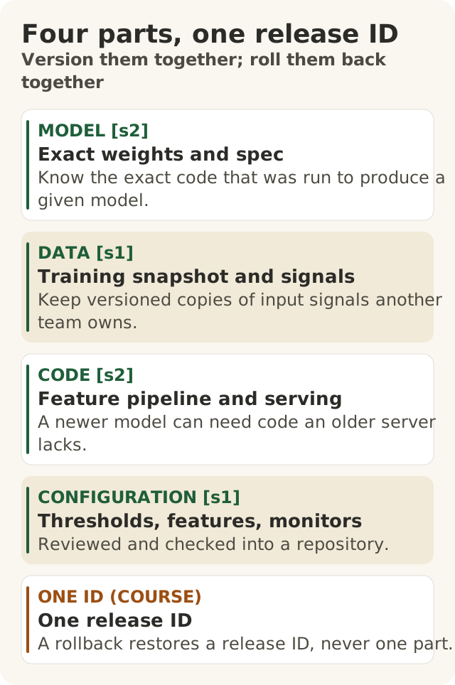
Figure data as text
Four parts, one release ID
| Part | What it shows |
|---|---|
| MODEL [s2] | Exact weights and spec. Know the exact code that was run to produce a given model. |
| DATA [s1] | Training snapshot and signals. Keep versioned copies of input signals another team owns. |
| CODE [s2] | Feature pipeline and serving. A newer model can need code an older server lacks. |
| CONFIGURATION [s1] | Thresholds, features, monitors. Reviewed and checked into a repository. |
| ONE ID (COURSE) | One release ID. A rollback restores a release ID, never one part. |
Misconception corrected: "Rolling back a model is the same as rolling back code."
Breck et al.: "a trained ML model needs production practices like a binary does, such as debuggability, rollbacks and monitoring", and one response unique to ML "is to roll back not the system code but the learned model".2 That is necessary, not sufficient. By Sculley et al.'s CACE principle ("Changing Anything Changes Everything"), behaviour is a joint function of weights, data, feature code and configuration; CACE applies "not only to input signals, but also to hyper-parameters, learning settings, sampling methods, convergence thresholds, data selection, and essentially every other possible tweak".1
The manifest
release: R13
model:   {id: fc-13, spec_commit: <hash>}        # Breck Model 1: know the exact code that produced it
data:    {train_snapshot: ds-2026-09, frozen_signals: [dealer-master@2026-09-30]}
code:    {feature_pipeline: fp-13, serving: sv-13, feature_schema: <hash>}
config:  {thresholds: cfg-13, monitor: mon-13, pages: [Dana Reyes], consumers: [parts, pricing]}
stop:    {who: [Dana Reyes, on-call forecast engineer], rollback_to: R12}
Each field has a source rationale:
- Model: "it's crucial to know the exact code that was run to produce a given learned model" (Model 1).2
- Data: for unstable data dependencies, "create a versioned copy of a given signal"; versioning "carries its own costs", such as "potential staleness".1
- Code: model and serving code drift. Breck et al.'s example: a newly trained model expects a new operation implementation, and "an older deployed server will not include Op0.2 and so will refuse to load the model" (Infra 6). Training and serving feature code can diverge (Monitor 3).2
- Config: reviewed and checked in; a manually set threshold "may be invalid" after an update.1
Course rule. Rollback is an atomic restore of a release ID. Serving checks that the incoming feature schema hash equals the model's expected schema and fails closed if not. Without that check, a mismatch that preserves the input shape could serve silently with skewed features.
Gate and stage
Infra 4: an automated system "must either bless the model or veto it"; test for slow degradation with loose thresholds against validation predictions, and for sudden drops by comparing "to the previous version of the model while setting tighter thresholds".2 Infra 6: turn up new models "gradually, running old and new models concurrently, with new models only seeing a small fraction of traffic, gradually increased as the new model is observed to behave sanely".2
Shankar et al.'s interviewees used stages named "test, dev, canary, staging, shadow, A/B", usually "between one and four". In shadow, predictions are generated live but not surfaced. With a feedback loop "it is impossible to evaluate the model in shadow mode because users do not interact with shadow predictions".3 They kept fallbacks ("either an old version or simple version") and kept "records of any change to production in case of a necessary rollback".3
What each stage establishes before labels mature (course reading). Shadow tests serving compatibility, schema conformance and output plausibility (Layers 1 and 2) on live inputs. It cannot estimate the effect of acting on the new scores, so with a feedback or intervention loop it says nothing about $y$ under the new policy. A live fraction bounds exposure and yields Layers 1 and 2 for that fraction; it yields Layer 3 only once labels for that fraction mature. With label delay $L$ (here six weeks) and stages shorter than $L$, no stage observes outcome quality. Advancing is then a gate decision by a named person on proxy evidence: allow, constrain (cap the fraction), hold (wait for labels or a person) or deny. Record the decision, the decider and the evidence it rested on; "no page" is absence of a detected problem, not a measurement of quality. Stages also cover only the conditions that occurred during them: Region 9 opened after the last stage.
Authority and rehearsal
NIST MANAGE 2.4: "Mechanisms are in place and applied, and responsibilities are assigned and understood, to supersede, disengage, or deactivate AI systems that demonstrate performance or outcomes inconsistent with intended use." MANAGE 4.3: incidents and errors are communicated, and processes for "tracking, responding to, and recovering from incidents and errors are followed and documented".4 Breck et al., Infra 7: "Because rolling back is an emergency procedure, operators should practice doing it normally, when not in emergency conditions."2
A rollback restores serving state; it does not retract decisions already taken or labels already influenced. The incident record lists predictions made by the withdrawn release so later training can exclude or reweight them (course practice; see feedback loops below). Nor does it make the prior release valid under the current $q$: restoring train_snapshot pins what the model learned from, while live inputs stay current. If the shift that paged (here, an unseen region) is still present, the restored release is outside its own reference too, and its Layer 1 will say so.
Scoring readiness
Breck et al.'s rubric: 28 tests in four sections (data, model, infrastructure, monitoring). Per test, 0.5 points if run manually with results documented and distributed, 1 point if automated and repeated. With $S_j$ the sum for section $j$,
\text{ML Test Score} = \min_{j \in \{\text{data, model, infra, monitor}\}} S_j .They chose the minimum "because we believe all four sections are important". Their Table V reads a score in $(3,5]$ as "Strong levels of automated testing and monitoring, appropriate for mission-critical systems".2 They interviewed 36 teams; integration testing and training/serving skew were among the least implemented.2
At Big Widget (made up)
Day 16: the on-call engineer restores model: fc-12 only. fp-13 still emits dealer_region; fc-12's expected schema hash differs; serving rejects; the 300 stop holds orders above the planner's cap. Full restore of R12 (fc-12, fp-12, sv-12, cfg-12 incl. mon-12) succeeds; the monitor's reference returns to R12's. The incident record lists R13's Region 9 forecasts for exclusion review. R12 never saw Region 9 either, so the holder keeps the constraint: R12 forecasts Region 9, but orders above the planner's cap still wait for a person until Region 9 labels show R12 inside its bounds there. The constraint carries an owner (the holder) and a review trigger (first Region 9 labels, from day 57), so it cannot persist unreviewed.
3. Hidden technical debt and its controls
Misconception corrected: "The model is most of the system."
Sculley et al.: "developing and deploying ML systems is relatively fast and cheap, but maintaining them over time is difficult and expensive"; this debt "may be difficult to detect because it exists at the system level rather than the code level".1 Figure 1: "Only a small fraction of real-world ML systems is composed of the ML code". They suggest "a mature system might end up being (at most) 5% machine learning code and (at least) 95% glue code" (an estimate from experience).1
Entanglement (CACE)
For a model on features $x_1,\dots,x_n$: "If we change the input distribution of values in $x_1$, the importance, weights, or use of the remaining $n-1$ features may all change." This holds "whether the model is retrained fully in a batch style or allowed to adapt in an online fashion".1
Controls named in the paper: isolate models and serve ensembles where sub-problems decompose (with the caveat that improving one component can worsen the ensemble if errors become correlated), or detect "changes in prediction behavior as they occur", with slice-by-slice metrics.1 Breck et al. make the second a release gate with incremental per-slice thresholds against the previous release (Model 6).2 Underused features add exposure; "exhaustive leave-one-feature-out evaluations" find them.1
Big Widget: fp-13 added dealer_region; fc-13's reliance on order-history features shifted, which inflated forecasts for low-history dealers. A per-slice diff of fc-13 against fc-12 on the low-history slice, before day 0, is the control.
Feedback loops
Direct: a model "may directly influence the selection of its own future training data"; the paper notes bandit algorithms are the theoretically correct framing but "do not necessarily scale well", and suggests mitigation by "some amount of randomization" or "isolating certain parts of data from being influenced by a given model". Hidden: "two systems influence each other indirectly through the world", possibly between "completely disjoint systems". Both are harder to detect "if they occur gradually over time".1
Course formalisation. Let pricing act on forecasts, $a_{d,w} = g(\hat y_{d,w})$, and let demand respond to price, $y_{d,w} \sim P(y \mid x_{d,w}, a_{d,w})$. Training on $(x, y)$ pairs collected under $g \circ f_t$ teaches $f_{t+1}$ a mixture of demand and the effect of $f_t$'s own forecasts. The control: a randomly chosen set of dealers $H$ for which $a_{d,w}$ does not depend on $\hat y$, in line with the paper's randomisation and isolation controls, which it offers for direct loops; applying them to this hidden loop is the course's step.1 Partition $H = H_{\text{train}} \cup H_{\text{eval}}$ by dealer: $H_{\text{train}}$ supplies loop-free training data, $H_{\text{eval}}$ is never trained on and estimates quality free of the loop. Being outside the intervention loop does not by itself make data a held-out test set. Shadow evaluation cannot substitute, since shadow predictions do not act on the world.3
Undeclared consumers (visibility debt)
Outputs written "to files or logs that may later be consumed by other systems" acquire consumers that are "silently using the output of a given model as an input to another system", creating "a hidden tight coupling"; they "may create hidden feedback loops". Detection is hard "unless the system is specifically designed to guard against this case, for example with access restrictions or strict service-level agreements (SLAs)". "In the absence of barriers, engineers will naturally use the most convenient signal at hand."1 For data dependencies generally, the paper recommends tooling that annotates data sources and features so "dependency trees can be fully resolved".1 Breck et al. put the reverse duty on consumers: "make sure that the dependent team knows your team is using the data" (Monitor 1).2
Big Widget: finance's warranty-reserve sheet reads the forecast log. Control: log access restricted to the manifest's consumers list, each notified before a release.
4. The operating plan as an artifact
| Part | Content | Evidence it works |
|---|---|---|
| Hold card (from 300) | $h$, $\Theta$, stop; provenance label | 300 dry-run receipts |
| Monitoring plan | Layers 1 to 3, statistic, reference version, one page per layer, route | Measured alert rate; a replayed shift that pages25 |
| Release manifest | One release ID over model, data, code, config; stages; gate; who can stop | A gate veto and a dry rollback restoring the prior release ID24 |
| Debt register | Each entanglement, loop and consumer, with its control | Per-slice diff; hold-out set; access list1 |
The one-release-ID rule, the one-page-per-layer routing and the Layer 2 proxy are course practice, not results from the sources.
NIST: it is "incumbent on Framework users to continue to apply the MANAGE function to deployed AI systems as methods, contexts, risks, and needs or expectations from relevant AI actors evolve over time".4
The three yeses as gate states
The operating part of the AiGovOps Foundation's three yeses, taught in module 100.9 (Get to Yes · Stay at Yes · Recover to Yes; note to, at, to), with each gate answer one of allow (go ahead), constrain (only this far), hold (wait for a person) or deny (no), decided by a named person, never by the model or the monitor:
| Movement | Gate | Evidence it may rest on | What it does not establish |
|---|---|---|---|
| Get to Yes | Each stage advance of a release ID (Infra 4 bless/veto, then the holder's answer) | Gate tests, Layers 1 and 2 for the stage, dry rollback | Outcome quality, while labels are immature |
| Stay at Yes | Continuing operation | Layers 1 to 3 against the release's own reference; Layer 3 runs when labels land even with no page | That the replayed false-page rate still holds as $q$ moves |
| Recover to Yes | Hold, full rollback, affected-prediction list, root-cause fix | Labels (or an agreed, validated check) showing the restored or fixed release inside bounds on the failing slices; the holder's agreement | Stopping alone is not recovery; until the evidence exists the status is "not known yet", owned by the holder |
Receipts and records. A gate receipt holds no private content: decision, decider, time, release ID, policy and manifest hashes. Forecasts for named dealers, order data, the affected-prediction list and incident notes stay in the access-controlled work record that the receipt's hashes point to. A hash lets a stranger confirm a record has not changed; it does not show the record's content was correct, and it is not a licence to publish that content. In this module the receipt may be an unsigned decision record. Modules 400.8 and 400.9 build the verifiable receipt.
Readiness statements
Before asking the holder for a stage decision, the operator should be able to state each line, or state that it is not known yet and who owns closing it:
- I know the paging threshold per layer and the 300-card threshold $\theta_a$ each one measures.
- I know the combined rule's replayed false-page rate with its interval, or I record it as not known with an owner.
- I can restore the prior release ID atomically, with a dry rollback rehearsed outside an emergency.
- I know every consumer of the output, and each is in the manifest's
consumerslist. - I know who answers allow, constrain, hold or deny for each stage, and the evidence each answer rests on.
Limits of the evidence
- Shankar et al. is a preprint of 18 interviews; the authors call velocity, validation and versioning the variables that "govern success", an interview finding rather than a measured effect.3
- Rabanser et al.'s detection rates are for image data with simulated shifts.5
- Sculley et al. and Breck et al. report Google's experience as of 2015 and 2017.12
- No source gives a false-page rate for a dependent, multi-rule paging policy like mon-13; this module gives none either. It has to be measured by replay on the real system.
- An operating plan is checkable evidence of what is watched, who decides and how to restore a known-good release. It is not an assurance that the system is safe, and completing this module describes the learner's practice, not a system's assurance.
Further learning (not sources)
Opened 18 Nov 2026; not citations: Stanford CS 329S Machine Learning Systems Design (https://stanford-cs329s.github.io/); University of Washington CSE 599W Systems for ML (https://dlsys.cs.washington.edu/); University of Michigan EECS 598 Systems for Generative AI, Winter 2024, public repository, not verified as complete (https://github.com/mosharaf/eecs598/tree/w24-genai).