
Evaluations that hold up · Technical gear
You will be able to: design an evaluation for a Big Widget task (held-out data matched to the deployment distribution, a baseline, a harm-linked metric and an a-priori sample size from a power calculation); identify contamination and adaptive test-set reuse, and decompose a score drop on a same-process replication into adaptivity, distribution and generalization gaps; and report an eval with standard errors (naive, clustered and paired), decide whether a difference is distinguishable from noise or large enough to act on, and validate an LLM judge against independent human labels.
This module is as of November 2026. Results about particular models are dated to the papers that report them. Big Widget Company is made up, and every Big Widget number below is made up for teaching.
1. A replication that did not replicate
Setup
Recht, Roelofs, Schmidt and Shankar (arXiv 1902.10811; ICML 2019) formalise what a test score is supposed to estimate.1 For a classifier f̂ and a data distribution D, the population loss is
L_D(f̂) = E_(x,y)∼D [ 𝟙[f̂(x) ≠ y] ],
and a test set S drawn from D gives the estimate
L_S(f̂) = (1/|S|) Σ_(x,y)∈S 𝟙[f̂(x) ≠ y].
They state that this assumption, that a low L_S means similar performance on future draws from D, "underlies essentially all empirical evaluations in machine learning".1
They then collected new test sets S′ from a distribution D′ built to match D, by repeating the CIFAR-10 and ImageNet creation processes (same source pools, Flickr images from a similar time frame for ImageNet, and MTurk tasks modelled on the originals).1 The drop on S′ decomposes into three terms:1
L_S − L_S′ = (L_S − L_D) + (L_D − L_D′) + (L_D′ − L_S′) adaptivity gap distribution gap generalization gap
- Generalization gap (L_D′ − L_S′): pure sampling error, because S′ is independent of f̂. With 10,000 independent points, as in the new ImageNet set, a 95% Clopper-Pearson interval for accuracy is at most ±1%; at 99.99% it is at most ±2%. So "random chance alone cannot explain the accuracy drops".1
- Adaptivity gap (L_S − L_D): how much tuning against S makes L_S underestimate L_D. Hyperparameter tuning on the test set "introduces dependencies between the model f̂ and the test set S".1
- Distribution gap (L_D − L_D′): the systematic difference between the original and the replicated distribution, which "is not influenced by random effects".1
Results
Accuracy fell by 3 to 15 percentage points on CIFAR-10 and 11 to 14 on ImageNet (the paper writes these absolute drops as "%").1 Examples from their Table 1: ResNet-152, 78.3% → 67.0% top-1 on ImageNet; the best CIFAR-10 model, 98.4% → 95.5%.1
To separate adaptivity from distribution shift, they used many models. If later, more-tuned models gained mainly through adaptivity, new-set accuracy would show diminishing returns. Instead the fit is linear with slope above 1:1
acc_new ≈ 1.69 · acc_orig − 72.7% (CIFAR-10), acc_new ≈ 1.11 · acc_orig − 20.2% (ImageNet top-1),
with bootstrap 95% intervals on the slope of [1.63, 1.76] and [1.07, 1.19].1 The authors call adaptivity "an unlikely explanation" and point to the distribution gap.1 Supporting that, three ImageNet sampling strategies drawn from the same candidate pool, all correctly labelled, shifted average top-1 accuracy from −11.8% to +2.1% relative to the original validation set, a spread of about 14 points.1
Two limits the authors state themselves: the experiments "do not exclude all variants" of adaptive overfitting (for example, a roughly constant drop affecting all models equally), and testing that would need "a new test set that is truly i.i.d.", which motivates their "super hold-out" proposal.1
What it shows for an engineer: a point estimate on one test set measures that set. Small, undocumented choices in collection and labelling produce shifts far larger than the sampling error, and rankings can be stable while absolute scores are not.1
The misconception this corrects: "If the model never saw the test file, the score is clean." The new sets were independent of every model by construction, so the gap was not leakage, and the scores still fell well outside sampling error.1
2. Contamination and adaptive reuse
Taxonomy
Sainz et al. (arXiv 2310.18018; Findings of EMNLP 2023) define contamination broadly as "any breach in the strict control of datasets required by the experimental protocol", focusing on an LLM that processed a benchmark during pre-training.2 Their levels:2
| Type | What leaked | Consequence (as the paper states it) |
|---|---|---|
| Guideline | Annotation guidelines | Advantage, especially for zero- and few-shot evaluation |
| Raw text | Source text before annotation (e.g. Wikipedia-based datasets) | Partial information about the labels, e.g. entity boundaries |
| Annotation, evaluation split | Test labels | "the experiment is completely invalidated" |
| Annotation, train/dev split | Training labels | Comparisons with models trained on those splits survive; zero-/few-shot claims are invalidated |
They place contamination at three stages: pre-training, supervised fine-tuning, and after deployment, where API-served models "have been iteratively improved with user input, leading to evaluation data exposure".2 HELM (Liang et al., arXiv 2211.09110; TMLR 2023) widens the definition to exposure to the evaluation distribution, and distinguishes strong from weak contamination by how much of that distribution the model saw.3
Detection
- Open training data: string-matching against the corpus. Sainz et al. propose reporting overlap as "the percentage of the benchmark that can be found in the pre-training dataset".2
- Closed training data: probe memorisation. Adapting Carlini et al., they define an example s as extractable from dataset d by model m if some k preceding examples, used as a prompt, make m generate s; the degree of contamination is the fraction of extractable examples.2
- Absence of evidence: whether a lack of memorisation ensures a model was not trained on a benchmark is a question that, in their words, "remains to be solved".2 Report a negative probe as "not detected", not as "uncontaminated".
HELM states the practical position for most evaluators: with "uneven and usually limited information" on training, "we cannot verify whether the model was trained on the data we evaluate it on"; they flag disclosed contamination next to affected results.3
Adaptive reuse
Reuse is the adaptivity term from section 1. In Recht et al. it arises when researchers tune hyperparameters "directly on the test set".1 This course reads the mechanism (dependence between f̂ and S) more widely than hyperparameters: it is produced by whoever lets test results flow back into model, prompt or threshold selection, whether the model's builders, the evaluating team, or both. Updating weights is not required; choosing among prompts by test score is enough.
A one-look policy (course practice; the cited studies do not give a rule for repeated release decisions):
- A development set, used freely for prompt and hyperparameter work.
- A test set with n fixed by the power calculation (section 3), opened once for one release decision. The CI in section 4 is a fixed-n, single-look interval; it is not a stopping rule.
- If the decision is hold, do not append items to the same test set and recompute until the lower bound clears 0. Repeated looks with data-dependent stopping let test results feed back into the decision, the same dependence as the adaptivity term; and the section 4 interval was computed for a fixed n and one look, not for a procedure that chooses when to stop by looking. Retire the opened set into development, redo the power calculation, and draw a fresh test set from inputs disjoint from everything seen.
- Count attempts. The decision record lists every prior test set and its outcome. Logging an opening, or calling a rerun "a new release decision", does not restore independence. A fresh set gives each attempt a valid fixed-n interval; it gives no family-wise bound across attempts, so the chance of at least one false allow grows with the number of attempts. The decider sees the full count. If the plan needs a campaign-wide error bound, it needs an error-allocation rule written before the first attempt; this module does not supply one.
- A hidden super hold-out, opened rarely, to check whether reuse of the working test sets has crept in.
A group-sequential or other multiple-look design, with its error budget allocated before the first look, is a legitimate alternative. It is not taught here, and must be specified in the pre-registered plan by someone qualified to design it.
3. Design: data, baseline, metric, sample size
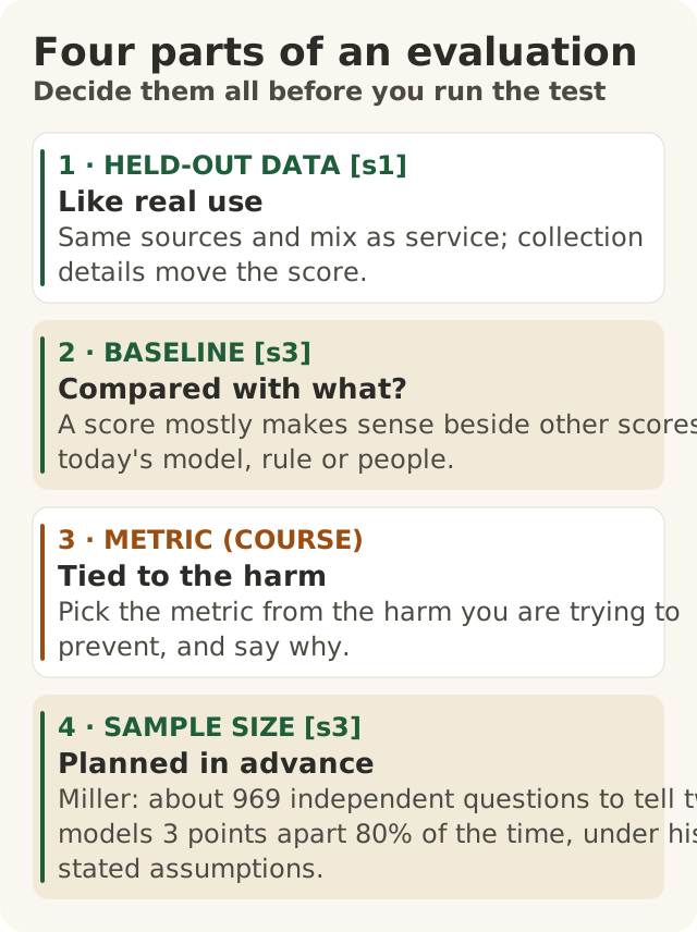
Figure data as text
Four parts of an evaluation
| Part | What it shows |
|---|---|
| 1 · HELD-OUT DATA [s1] | Like real use. Same sources and mix as service; collection details move the score. |
| 2 · BASELINE [s3] | Compared with what? A score mostly makes sense beside other scores: today's model, rule or people. |
| 3 · METRIC (COURSE) | Tied to the harm. Pick the metric from the harm you are trying to prevent, and say why. |
| 4 · SAMPLE SIZE [s3] | Planned in advance. Miller: about 969 independent questions to tell two models 3 points apart 80% of the time, under his stated assumptions. |
Why external benchmarks do not transfer
Section 1 shows replication shift; section 2 shows unverifiable contamination. HELM adds measurement conditions: before HELM, models had on average been evaluated on 17.9% of its 16 core scenarios, and prompting details produced "wild swings in accuracies", from 30% to 80% for the same model and scenario.3 Zheng et al. (arXiv 2306.05685; NeurIPS 2023 Datasets and Benchmarks) report that benchmarks like MMLU and HELM "cannot effectively tell the difference" between aligned chat models and their base models, though people strongly prefer the aligned ones.4
The misconception this corrects: "A public leaderboard score tells you how a model will do on your task." It is evidence about a different distribution, under different conditions, with unknown contamination.
The four design choices
- Held-out data from the deployment distribution. Sample from the inputs the model will serve, from a period disjoint from anything used in development. For drifting inputs, prefer a temporal split (most recent period) to a random split (course design advice).
- A baseline on the same items. Miller (arXiv 2411.00640, 2024, a preprint): a single model's score "usually does not have any inherent meaning".5 Run the incumbent (model, rule or human process) on the identical items so you can use a paired analysis (section 4).
- A metric tied to the harm. HELM targets seven metrics (accuracy, calibration, robustness, fairness, bias, toxicity, efficiency) for each core scenario "to the extent possible", which it reports as 87.5% of the time: a reminder that accuracy is one column of many, and that an evidence matrix should show its empty cells.3 Choose the metric whose errors correspond to the harm, and report the others you need as guards.
A sample size from a power calculation, fixed in advance. For a paired comparison with significance level α, power 1 − β and minimum detectable effect δ, Miller gives5
n = (z_α/2 + z_β)² (ω² + σ²_A/K_A + σ²_B/K_B) / δ²,
where ω² = Var(x_A) + Var(x_B) − 2Cov(x_A, x_B) is the variance of the per-question mean difference, σ²_A and σ²_B are the within-question (resampling) variances, and K_A, K_B the number of samples per question. With σ²_A = σ²_B = 0, ω² = 1/9, δ = 0.03, α = 0.05 and β = 0.20, this gives n ≈ 969, so he suggests new evals "should contain at least 1,000 questions".5 Inverted, the same equation gives the minimum detectable effect for a fixed n; in his example with n = 198, raising K from 1 to 10 cuts it from 13.2% to 7.5%.5
Big Widget: the safety-claim flagger (made up)
| Choice | Decision |
|---|---|
| Task | Flag free-text warranty claims that may describe a safety defect, for same-day engineer review |
| Harm | A missed safety claim (false negative); secondarily, alert fatigue from false flags |
| Primary metric | Recall on safety claims ("catch rate"), denominator = engineer-labelled safety claims |
| Guard metric | False-flag rate on non-safety claims, with a ceiling the safety lead sets |
| Baseline | Current keyword rule, scored on the same claims |
| Test set | All claims from the most recent full quarter; two engineers label independently before any model run; disagreements adjudicated; claims touched in prompt development excluded; stored outside the prompt writers' access |
| Sample size | Planned for the positive class: at a prevalence of about 3%, 10,000 claims hold about 300 safety claims |
| Decider | The safety lead signs the plan before the test set is opened, makes the release decision, and is the named person who can release a hold; the model and the evaluation pipeline decide nothing |
| Release rule (pre-registered, one look) | Allow (replace the rule) only if the paired 95% CI for recall(model) − recall(rule) has a lower bound above 0 and the guard holds. If the CI spans 0: hold; the keyword rule stays, and any further attempt needs a fresh test set under the one-look policy (section 2). If the upper bound is below 0 or the guard fails: deny |
4. Uncertainty, comparisons and judges
Standard errors
Treating eval questions as drawn from a super-population, Miller gives the CLT standard error of the mean score5
SE = √( Var(s) / n ), and for binary scores SE = √( s̄(1 − s̄) / n ),
with CI₉₅ = s̄ ± 1.96 · SE.5 He recommends reporting n and the SE in parentheses beside each score.5 Big Widget (made up): 270/300 safety claims caught, s̄ = 0.90, SE = √(0.9 · 0.1 / 300) ≈ 0.0173, CI₉₅ ≈ [0.866, 0.934].
Clustering. When questions are drawn in groups (several questions per passage; one question in many languages), independence fails and the naive SE is inconsistent. Miller's clustered SE adds the within-cluster cross-terms,
SE_clustered = ( SE²_CLT + (1/n²) Σ_c Σ_i Σ_(j≠i) (s_i,c − s̄)(s_j,c − s̄) )^½,
and on real eval data scored with Anthropic models it came out up to about 3× the naive SE (DROP: 1.34 vs 0.44, ratio 3.05).5 Claims from the same vehicle or dealer are a plausible cluster at Big Widget; recall also sits on top of the labelling step, which this formula does not cover.
Paired differences
For two models on the same n items, with d_i = s_A,i − s_B,i, Miller's paired SE is5
SE_paired = √( Var(d) / n ), where Var(μ̂_A−B, paired) = Var(μ̂_A−B, unpaired) − 2 Cov(x_A, x_B)/n.
Because models tend to agree on which items are hard, the covariance is usually positive, so pairing is "a 'free' reduction in estimator variance"; he recommends it "wherever practicable".5 In his fictional table, MATH gives +2.5% (SE 0.7%), CI (+1.2%, +3.8%), significant; MGSM gives −2.7% (SE 1.7%), CI (−6.1%, +0.7%), not significant at 5%.5
Worked Big Widget example (made up): 200 claims scored by models A and B. B is right where A is wrong on 14; A is right where B is wrong on 10; elsewhere they agree. Here we want B − A, so take d_i = s_B,i − s_A,i (the reverse of the convention above; a positive d̄ favours B, and the variance is the same either way). Then d̄ = (14 − 10)/200 = +0.020, the sample variance of d is (24 − 200 · 0.020²)/199 ≈ 0.1202, SE_paired = √(0.1202/200) ≈ 0.0245, and CI₉₅ ≈ +2.0 ± 4.8 points = (−2.8, +6.8). Honest report: "B − A = +2.0 points (SE 2.5; 95% CI −2.8 to +6.8; n = 200, paired). The data do not distinguish the two models." That is not evidence of equivalence. Under the release rule this is a hold, and the next attempt needs a fresh test set (section 2). Whether a difference that is distinguishable is worth acting on is the release rule's job (section 3), and the safety lead's decision, not the test's.
The misconception this corrects: "A two-point gain on a benchmark is a real improvement." With n = 200 and this discordance, a 2-point gain is well inside the noise.
Validating an LLM judge
Zheng et al. study three judge formats (pairwise comparison, single-answer grading, reference-guided grading) with 2023-era judges (GPT-4, GPT-3.5, Claude-v1).4 Measured failure modes:4
| Bias | Probe | Result (as reported) |
|---|---|---|
| Position | Two similar answers, order swapped | Consistency: GPT-4 65.0%, GPT-3.5 46.2%, Claude-v1 23.8% (default prompt) |
| Verbosity | "Repetitive list" padding on 23 answers | Failure rate: Claude-v1 91.3%, GPT-3.5 91.3%, GPT-4 8.7% |
| Self-enhancement | Win rates vs humans | GPT-4 +10%, Claude-v1 +25% for themselves; the authors say their data cannot determine whether it is a bias |
| Maths grading | 10 questions, positions swapped (20 judgments) | GPT-4 failures: default 14/20, chain-of-thought 6/20, reference-guided 3/20 |
Agreement. They define agreement between two judge types as the probability that randomly chosen individuals of each type agree on a randomly chosen question.4 On first-turn MT-bench (58 expert labellers, mostly graduate students):4
| Setup | Chance (R) | GPT-4 (pairwise) vs human | Human vs human |
|---|---|---|---|
| S1: ties and position-inconsistent votes counted as ties | 33% | 66% | 63% |
| S2: non-tie votes only | 50% | 85% | 81% |
Agreement with humans rose "from 70% to nearly 100%" as the win-rate gap between the compared models grew, so the judge was least reliable on close pairs.4 And when experts who disagreed with GPT-4 were shown its judgment, they rated it reasonable in 75% of cases and changed their choice in 34%.4 This course reads that as a route by which a judge can contaminate the human labels it is checked against.
A validation protocol (course practice built on these results):
- Fix the decision unit and label set (single-output classification such as faithful/unfaithful, or pairwise preference) and the tie rule. Humans and judge label the same unit.
- Sample items stratified to include close calls and long outputs.
- Collect ≥ 2 independent human labels per item before anyone sees the judge's output.
- Run the judge; for pairwise judging, run both orders and count inconsistency as a tie, as Zheng et al. do.4
- Report matched estimators on a common sample: judge–individual-human agreement and human–human agreement over the same items, in the sense of Zheng et al.'s definition above, with chance, n and an interval. Agreement with human consensus on the subset where humans agree is a different, conditional quantity; label it as such if you report it at all.
- Retain the human-disagreement items. They are the hard cases; send them for adjudication and analyse them, do not filter them out.
- Read the disagreements by stratum. A named person records the judge's permitted role (allow: replace; constrain: pre-sort; deny: none), the evidence, and the date.
The misconception this corrects: "An LLM judge agrees with people." Agreement is task-, format-, tie-rule- and difficulty-dependent; it is a measured property of this judge on this task.
Big Widget (made up): binary faithfulness labels on 50 claim summaries. Two engineers agree on 44 (88%). The judge matches the engineers' consensus on 36 of those 44 (81.8%), but that is conditional on human agreement and excludes the hard cases, so it is not comparable with 88%. The matched estimator: on the 44 agreed items the judge matches both engineers 36 times and neither 8 times; on the 6 disputed items a binary judge matches exactly one engineer. Judge–engineer agreement is therefore (2 · 36 + 6)/100 = 78%, against 88% engineer–engineer, on the same 50 items. With n = 50 both intervals are wide, and the 100 judge–engineer comparisons are not independent (two per item). Most judge misses are long summaries marked "faithful": a reason to run a targeted verbosity probe, not proof of the local cause. Decision recorded: constrain (pre-sort only, not replacement), made and signed by the quality lead; the 6 disputed items go to adjudication.
5. The three yeses for an evaluation
The evaluation is evidence for a gate; it is not the gate. A named person decides at each stage. The Foundation's three yeses (Get to Yes, Stay at Yes, Recover to Yes) are a cycle, not a one-time approval.
- Get to Yes: a pre-registered plan (test-set provenance, baseline, metric and guards, power calculation, one-look release rule, the named decider) signed before the test set is opened, plus a "not checked" list, such as undisclosed vendor training data, in the way HELM flags contamination beside results.3 Each "not checked" line names an owner and a next check, or states that none is possible; a negative probe is "not detected", never "clean". The resulting allow is scoped to this model, task, test set and guard; it is not a blanket licence.
- Stay at Yes: after every fine-tune or prompt change (module 400.2), re-check on the development set; any new release decision gets a fresh test set under the one-look policy (section 2). Rotate the test set as inputs drift (module 400.4) and keep a super hold-out to detect creeping reuse.1
- Recover to Yes: on discovering a leak, the decider puts dependent releases on hold, and the affected results are voided where they were reported. Sainz et al. call for flagging published work whose conclusions contamination has compromised.2 Voiding is containment, not recovery: you are back at yes only after a fresh test set, a re-run, and a new decision on that evidence.
What you keep, and where:
- Work record (internal, access-controlled): the plan, the dated test-set description, the test items themselves, results with SEs and CIs, the judge validation and the disagreement items.
- Receipt (shareable): decision (allow · constrain · hold · deny), deciding role, date, and hashes of the plan and test-set description. It never carries prompts, outputs, claims, test items or personal data, and a hash is not a licence to disclose what it was computed from. Module 400.8 covers offline verification. A verified receipt shows the recorded decision has not been altered since signing; it says nothing about whether the model's outputs are correct.
Words to know: population loss, adaptivity gap, distribution gap, generalization gap, contamination (guideline, raw-text, annotation), extractability, standard error, clustered standard error, paired difference, minimum detectable effect, power, judge agreement, position bias, verbosity bias, development set, one-look policy, matched agreement estimator, not detected, not checked, work record, receipt.