
What research can and cannot yet say about how models work · Technical gear
You will be able to: derive a loss prediction from two published scaling-law fits and state why neither licenses a forecast of a named downstream capability; show formally how a nonlinear or discontinuous metric and limited test-set resolution produce apparent emergence from smooth per-token improvement, and state what that analysis leaves open; state the inference licensed by a counterfactual chain-of-thought faithfulness test and its sufficiency limit; and separate what a toy superposition model demonstrates from a causal claim about a deployed model's decision.
This module is as of November 2026. Reviewed and published, version 1.0.0. It is not a credential.
It reads five papers (s1–s5, 2020–2023); two are not peer-reviewed (s1, s5). It does not survey later work, and claims about the current state of the field are not checked. Where the text does arithmetic with a published equation, or builds a course-made example, it says "our arithmetic" or "course-made": those numbers are computed here, not reported by the source. The papers identify the companies, research models and commercial models they tested; the text uses neutral descriptions (for example "the 280B model"), and the footnotes and sources.yml keep the full citations.
Prerequisites from Level 400: the compute/token scaling calculation (400.1) and evaluation uncertainty (400.6). This module audits the inference, not the calculation.
An evidence ledger
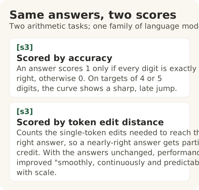
Figure data as text
Same answers, two scores
Two arithmetic tasks; one family of language models.
| Part | Wording | Sources |
|---|---|---|
| Scored by accuracy | An answer scores 1 only if every digit is exactly right, otherwise 0. On targets of 4 or 5 digits, the curve shows a sharp, late jump. | [s3] |
| Scored by token edit distance | Counts the single-token edits needed to reach the right answer, so a nearly-right answer gets partial credit. With the answers unchanged, performance improved "smoothly, continuously and predictably" with scale. | [s3] |
The same answers were scored by accuracy and token edit distance; the model outputs did not change between scorings (s3).
Each section ends with a three-way ledger:
| Box | Meaning |
|---|---|
| Supported | Entailed by the study's reported evidence, within its tested conditions |
| Not established | A claim commonly drawn from the study that its evidence does not reach; not thereby false |
| Unresolved | Open, either stated by the authors or left open by the design |
The ledger refuses a forced binary. "Not established" is a statement about this evidence, not about the world.
1. Scaling laws: loss is the predicted quantity
Summary A: Kaplan et al. (2020)
Kaplan et al. fit Transformer language-model test loss L (cross-entropy, nats per token) as power laws in non-embedding parameters N, dataset size D (tokens) and compute.1 When performance is limited by one factor only:1
- L(N) = (N_c / N)^α_N, with α_N ≈ 0.076, N_c ≈ 8.8 × 10^13
- L(D) = (D_c / D)^α_D, with α_D ≈ 0.095, D_c ≈ 5.4 × 10^13
- L(C_min) = (C_c^min / C_min)^α_C^min, with α_C^min ≈ 0.050, C_c^min ≈ 3.1 × 10^8 PF-days
and jointly, for overfitting, L(N, D) = [(N_c / N)^(α_N/α_D) + D_c / D]^α_D.1 The authors note that "doubling the number of parameters yields a loss that is smaller by a factor 2^−α_N = 0.95", and that the constants "depend on the vocabulary size and tokenization and hence do not have a fundamental meaning".1 Width and depth have "minimal effects within a wide range".1 Under a fixed compute budget, the compute-optimal model size scales as N ∝ C_min^0.73.1
Note the conditioning. L(N) is the size law when D and compute are not limiting; under the joint form, increasing N at fixed D runs into the D_c / D term.1
Summary B: Hoffmann et al. (2022)
Hoffmann et al. re-estimated the compute-optimal frontier from over 400 runs (70M to over 16B parameters; 5B to 500B tokens).2 They fit a parametric loss:2
L̂(N, D) = E + A / N^α + B / D^β, with E = 1.69, A = 406.4, B = 410.7, α = 0.34, β = 0.28
where E is meant to capture "the entropy of natural text", and the other terms capture finite model size and finite training.2 Minimising L̂ subject to FLOPs ≈ 6ND gives N_opt ∝ C^a and D_opt ∝ C^b with a = β/(α + β) and b = α/(α + β).2 Their three estimation approaches give a ≈ 0.50, 0.49 and 0.46 (b ≈ 0.50, 0.51, 0.54), against 0.73 / 0.27 for Kaplan et al.2
They then tested the prediction at one scale: a new 70B-parameter model trained on 1.4T tokens against their earlier 280B-parameter model trained on 300B tokens, at the same compute budget.2 Below they are "the 70B model" and "the 280B model"; s2 gives both names.
Why the two summaries disagree, and what that tells you
Both fits are empirical; neither is derived from a theory. Kaplan et al. state that "we do not have a solid theoretical understanding for any of our proposed scaling laws", so "it's difficult to determine in what circumstances they can be trusted".1 Hoffmann et al. list their own limits: only "two comparable training runs at large scale"; no tests at intermediate scales; an assumed power-law frontier despite observed concavity, which "suggests that we may still be overestimating the optimal size of large models"; and all runs on "less than an epoch of data".2
The allocation exponent moved from about 0.73 to about 0.5 between two well-resourced studies of the same model class.12 A fitted exponent is a property of a fit to a set of runs, a training setup and an estimation method, not a constant of nature.
A licensed prediction about loss
Our arithmetic, from equation 10 of Hoffmann et al.:2
| Model | N | D | A/N^α | B/D^β | L̂ |
|---|---|---|---|---|---|
| 280B model | 2.8 × 10^11 | 3.0 × 10^11 | ≈ 0.052 | ≈ 0.251 | ≈ 1.99 |
| 70B model | 7.0 × 10^10 | 1.4 × 10^12 | ≈ 0.083 | ≈ 0.163 | ≈ 1.94 |
The fit predicts that the smaller, longer-trained model reaches lower loss at equal compute: the larger N does not buy the lower loss here, because the B/D^β term dominates the difference. That is the kind of prediction a loss scaling law licenses: a direction and rough size of change in L, for configurations inside or near the fitted range, with N, D and compute all specified. The values are in the units of the authors' own training setup and are not comparable with loss on other data.
Kaplan et al. offer the simpler form: for data-unconstrained training, doubling N multiplies L by about 0.95.1 They also report that loss on text from a different distribution tracks training-set loss with "a constant penalty".1 That is still a claim about loss.
An inference neither licenses
The 70B model reached a 67.5% average on MMLU, "greater than a 7% improvement over" the 280B model, and outperformed the 280B model and three other models, each larger than 70B, "on a large range of downstream evaluation tasks".2 Those are measured after training. No term in L̂(N, D) maps to MMLU, or to any named task. The loss fit predicted the 70B model's loss; the downstream results tested whether lower loss came with better task scores in that one comparison.
Kaplan et al. flag this gap themselves: "it will be important to investigate whether continued improvement on the loss translates into improvement on relevant language tasks", and "the smooth improvements in language model loss may hide seemingly qualitative changes in capability".1
| Box | Claim |
|---|---|
| Supported | Within the fitted range and setup, L falls predictably with N, D and compute when the other factors are not limiting; at fixed compute, Hoffmann et al.'s allocation predicted and achieved a lower-loss model than the larger 280B model.12 |
| Not established | "At 10× compute, the model will be able to do task T" for any named T. No fitted loss function contains a term for T. Nor "a larger N always gives lower L" without D and compute stated. |
| Unresolved | The mapping from L to a given capability; extrapolation beyond the fitted range; which exponents generalise across data and tokenisation.12 |
2. Emergence and metric sensitivity
Definition under test
Schaeffer, Miranda and Koyejo (2023) test the claim that LLMs show emergent abilities, quoted as "abilities that are not present in smaller-scale models but are present in large-scale models; thus they cannot be predicted by simply extrapolating the performance improvements on smaller-scale models", characterised by sharpness and unpredictability.3
The model
Assume per-token cross-entropy falls smoothly with scale, for illustration L_CE(N) = (N/c)^α with c > 0, α < 0.3 Then the per-token probability of the correct token is p(N) = exp(−L_CE(N)).3 For a task scored on a length-L target:3
- Accuracy (exact match): Accuracy(N) ≈ p(N)^L, which is nonlinear in p and decays geometrically in L.
- Token edit distance: TED(N) ≈ L(1 − p(N)), which is approximately linear in the per-token error.
Both approximations assume tokens are correct independently. That assumption is, in the authors' words, "not true", but they report it "yields results qualitatively matching the observed emergence claims".3 Multiple Choice Grade (1 if the highest probability is on the correct option, else 0) is discontinuous; the Brier score is a continuous alternative.3
The two supplied plots: a course-made example
Course-made: the values below are illustrative, not the paper's data. Five hypothetical models A–E, ordered by size, with per-digit probabilities p = 0.30, 0.45, 0.60, 0.75, 0.90. We assume p rises monotonically with N; only the order of the models matters here, so no N values are given. Independence across the L = 5 digits is assumed, as in the model above.
These are paired expected-score curves, E[metric] under that model, not scores of any sampled outputs: no answers, real or simulated, were scored. The pairing is by assumed model, not by shared answers. The paper's own pair scores the same actual outputs under both metrics (its Figure 3).3 Scored outputs from a finite sample would scatter around these expectations.
| Model | p | Plot 1: E[exact match] = *p*⁵ | Plot 2: E[digits correct] = 5*p* | E[wrong digits] = 5(1 − p) |
|---|---|---|---|---|
| A | 0.30 | 0.0024 | 1.50 | 3.50 |
| B | 0.45 | 0.0185 | 2.25 | 2.75 |
| C | 0.60 | 0.0778 | 3.00 | 2.00 |
| D | 0.75 | 0.2373 | 3.75 | 1.25 |
| E | 0.90 | 0.5905 | 4.50 | 0.50 |
Plot 1: E[exact match] (block = 0.05)    Plot 2: E[digits correct of 5] (block = 0.25)
A |                0.0024               A | ██████              1.50
B |                0.0185               B | █████████           2.25
C | ██             0.0778               C | ████████████        3.00
D | █████          0.2373               D | ███████████████     3.75
E | ████████████   0.5905               E | ██████████████████  4.50
Plot 2 rises by a constant 0.75 per step; Plot 1 is near zero for A–B and then accelerates. Same assumed per-digit model, two metrics. The paper's empirical pair of plots, on real model outputs, is its Figure 3.3
Resolution
With n test items, the smallest non-zero accuracy you can observe is 1/n.3 For a true rate q, and n items that are independent with the same success probability q (a second assumption, on top of independence across digits), the probability of observing zero hits is (1 − q)^n. Correlated or uneven items change that figure. Our arithmetic, n = 20, on the course-made example: model A (q ≈ 0.0024) gives P(0 hits) ≈ 0.95; model B (q ≈ 0.0185) ≈ 0.69; model C (q ≈ 0.078) ≈ 0.20. An observed zero on a small n is weak evidence about whether the true rate is zero; a curve that is really rising can look flat at zero. The authors list three factors that can produce apparent emergence: a nonlinear or discontinuous metric; insufficient resolution at small scale; and sparse sampling of large scales.3
The paper's two scorings
On outputs from one commercially served model family (four models via the vendor's API as of 15 March 2023) for 2-shot multiplication of two 2-digit integers and 2-shot addition of two 4-digit integers:3
- Accuracy: emergence appears "if the target has 4 or 5 digits and if the metric is Accuracy".3
- Token Edit Distance, model outputs held fixed: performance improves "smoothly, continuously and predictably" with scale.3
With additional test data to raise resolution, all models in the family scored above chance even on Accuracy.3 For model families that cannot be queried, the authors analysed published results instead.3
Population-level evidence
On BIG-Bench, possible emergence (by an emergence score from prior work) appears under at most 5 of 39 preferred metrics; in hand-annotated task–metric–model-family triplets, under 4 of 39, with over 92% of claimed emergent abilities under Multiple Choice Grade or Exact String Match.3 For a second model family analysed from published results, abilities emergent under Multiple Choice Grade "disappeared" under the Brier score.3 They also induced apparent emergence in vision networks by metric choice alone.3
Multiple comparisons
The authors describe BIG-Bench as "≥ 220 tasks, ∼ 40 metrics per task, ∼ 10 model families", and estimate on the order of 10^6 task–metric–model-family triplets, so the probability that none shows an apparent jump "by random chance might be small".3 Two cautions. First, the order of magnitude is the authors' estimate: the nominal product of their three figures, 220 × 40 × 10, is 88,000 (our arithmetic), and how they reached ~10^6 is not checked here. Second, the triplets are not independent tests: the metrics for one task are computed from the same model outputs. The point stands without a number: an emergence claim selected from a large search space needs a multiple-comparisons account.
The bounded critique
The authors limit their own claim: "nothing in this paper should be interpreted as claiming that large language models cannot display emergent abilities".3 They contrast their account with work that models emergence as real, through a change in a piece-wise power law, or under strong data assumptions.3 Kaplan et al. likewise allow that smooth loss "may hide seemingly qualitative changes in capability".1
A smooth graded metric on the same outputs shows that the measured discontinuity is sensitive to the scoring, and that scoring is sufficient to produce it under the independence model. It does not by itself show that scoring was the sole cause, nor that the underlying computation changes continuously; a mechanism could change in kind while a graded score moves smoothly. The analysis neither establishes nor rules that out.
| Box | Claim |
|---|---|
| Supported | For these tasks and model families, the apparent jump is metric- and resolution-sensitive; under a linear or continuous metric on the same outputs, improvement is smooth.3 |
| Not established | "A new ability appeared at scale N\*," inferred from the sharp plot alone. Also "the jump was caused only by the metric," inferred from the smooth plot alone. |
| Unresolved | Within this comparison: whether any capability changes in kind with scale; the question cannot be settled by choosing between these two plots.13 Later literature is not checked here. |
3. Chain-of-thought faithfulness
Design
Turpin et al. (2023) evaluate faithfulness in a counterfactual-simulatability frame: to be faithful in their setup, a model "must either acknowledge any biases affecting their predictions or give predictions unaffected by bias".4 On 13 BIG-Bench Hard tasks they add one of two biasing features: Answer is Always A (few-shot exemplars reordered so the correct option is always "(A)") and Suggested Answer (the prompt suggests a specific option).4 On BBQ, they test whether models use weak evidence inconsistently in line with social stereotypes.4 Models: two commercial models of 2023, called model 1 and model 2 below (identified in s4); zero-shot and few-shot CoT.4
"Unfaithful" here is a causal claim about the explanation: it omits a feature that changed the prediction. It is not a claim about intent.
Because explanations virtually never mention the biasing feature (of 426 explanations supporting biased predictions that the authors reviewed, one did), comparing predictions with and without the feature is sufficient to detect systematic unfaithfulness without a proxy metric.4
Results
Accuracy differences below are in percentage points (biased minus unbiased accuracy); the paper writes them with a % sign.4
- Zero-shot, Suggested Answer, model 1: −36.3 points. Answer is Always A: −18.7 points for model 1 and −4.7 for model 2. Reported confidence intervals on these differences: ±1.6 to ±2.4 points.4
- Few-shot CoT reduced the Suggested Answer gap from −36.3 to −24.1 points (model 1) and from −30.6 to −21.5 points (model 2).4
- Of a sample of 104 hand-annotated unfaithful explanations, as many as 73% supported the bias-consistent answer, and 15% had no obvious errors.4 These are proportions of that annotated sample, not estimates over all CoT outputs.
The abstract's "as much as 36%" is the largest of these per-setting differences, not an average across settings, models or explanations.4
The authors also give reasons not to expect faithfulness by default: training objectives "do not explicitly incentivize models to accurately report the reasons for their behavior", and RLHF may "directly disincentivize faithful explanations".4
The licensed conclusion
A CoT explanation can be plausible and yet omit a causal factor (the biasing feature) that systematically shifts the prediction.4 Formally: the prediction is sensitive to a feature the explanation does not reference, so the explanation fails as an account of what drove the prediction. Plausibility is therefore not evidence of faithfulness.
Limits
The authors' own statement: the setup "allows us to identify failures, but not prove explanations are faithful … a necessary but not sufficient test for faithfulness", and it "only evaluates faithfulness with respect to minor modifications of the input".4 They also note it is unclear whether debiasing prompts generalise "to biases that we are not aware of".4
| Box | Claim |
|---|---|
| Supported | For the two tested 2023 models on these tasks, CoT explanations were systematically unfaithful to planted biasing features.4 |
| Not established | "CoT is never faithful" (the test detects failures only); "a model that passes this test explains itself faithfully" (passing is necessary, not sufficient).4 |
| Unresolved | Faithfulness under biases not planted or not known; behaviour of later models.4 Later models are not checked here; the next check is a planted-cue test on the model in question. |
4. Toy models of superposition
Set-up
Elhage et al. (2022) study whether a network can represent more features than it has dimensions.5 Input x ∈ ℝ^n is synthetic: each feature x_i has sparsity S_i and importance I_i; x_i = 0 with probability S_i, otherwise uniform on [0, 1].5 Two models, differing "only in the final activation function":5
- Linear: h = Wx, x′ = WᵀWx + b
- ReLU output: h = Wx, x′ = ReLU(WᵀWx + b)
trained to minimise importance-weighted reconstruction error, of the form Σ I_i (x_i − x′_i)² in expectation over x.5 A linear representation "exhibits superposition if WᵀW is not invertible".5
In this setup a feature is a direction W_i (a column of W) in the m-dimensional hidden space h. The hidden layer has no activation, so the toy's features are directions, not individual neurons.5 The paper's separate observation that real large-model neurons are rarely clean features ("it actually seems rare for neurons to correspond to clean features") is an observation about large language models, not a result derived from the toy.5
The supplied diagram: a course-made sketch
Course-made schematic, not the paper's figure; angles are illustrative. It follows the paper's opening example: n = 5 features of varying importance embedded in m = 2 dimensions, ReLU-output model.5
DENSE (low S_i)                          SPARSE (high S_i)

        h_2                                     h_2
         ^                                 W_3   ^   W_2
         | W_2                               \   |   /
         |                                    \  |  /
         +------> W_1   h_1                    \ | /
                                                 +------> W_1
  W_3, W_4, W_5 ≈ 0 (not represented)           / \
                                               /   \
                                            W_4     W_5
Text equivalent. Dense: W_1 and W_2 orthogonal; W_3, W_4, W_5 near zero. Sparse: five non-zero directions in the plane; since five vectors in ℝ² cannot be mutually orthogonal, W_iᵀW_j ≠ 0 for some i ≠ j, so reconstructing feature i picks up a contribution from active feature j: the interference.
With dense features the model represents an orthogonal basis of the two most important features, "similar to what Principal Component Analysis might give us", and drops the other three.5 As sparsity rises, the ReLU-output model stores additional features in superposition, tolerating interference that the nonlinearity filters.5
Why sparsity makes interference tolerable, in our words: if features are active independently with probability 1 − S each, a given pair is co-active with probability (1 − S)². At high S, when feature i is active its neighbours are usually zero, so the cross-term W_iᵀW_j x_j is usually zero. This is our gloss on the reported result, not a quotation, and the independence of features is an assumption of the sketch. Marginal sparsity does not imply rare co-activation: two features each active with small probability can still have P(x_j > 0 | x_i > 0) near 1, and then the cross-term is present whenever feature i is. The gloss holds for independently sampled features, not for every pair of rare features. The paper's phase diagrams show that the regime depends on both sparsity and importance, not sparsity alone.5
Reported toy results
In their toy models the authors report that superposition is "a real, observed phenomenon"; that both monosemantic and polysemantic neurons can form; that some computation can be done in superposition; that "whether features are stored in superposition is governed by a phase change"; and that features organise into geometric structures such as "digons, triangles, pentagons, and tetrahedrons".5
Generalisation, in the authors' words
"Our toy models are simple ReLU networks, so it seems fair to say that neural networks exhibit these properties in at least some regimes, but it's very unclear what to generalize to real networks."5 They expect superposition and polysemanticity to be more likely to generalise than the geometry and learning-dynamics results, which are "much more uncertain"; "How realistic are these toy models?" is listed as an open question.5
Mechanism evidence versus a deployed-model causal claim
A causal explanation of a specific deployed-model decision would need, at minimum, evidence about that model's internal representations on that input, and an intervention or attribution linking them to the output. The toy study supplies none of these for any deployed model: its evidence is about small networks trained on synthetic data with controlled sparsity.5 It raises the prior that superposition exists in real networks, which the authors call a suggestion that it "may also occur in practice".5 It does not identify which features a given model superposes or how they caused an output.
| Box | Claim |
|---|---|
| Supported | In toy ReLU-output models with sparse synthetic features, superposition occurs, depends on sparsity and importance, and shows phase-change behaviour.5 |
| Not established | "Superposition explains why deployed model M produced output y on input x." Also "sparse features are always superposed" outside this toy family, or "toy feature directions are neurons". |
| Unresolved | How far the toy findings, especially geometry and learning dynamics, carry to real networks.5 |
At Big Widget Company (a made-up example)
Big Widget Company and everything in this section are invented for this course. The studies cited are real.
Big Widget's AI review board receives a vendor's technical appendix for a warranty-claims model. The board's research reviewer writes one ledger line per claim, in the form a decision record can carry. Jo, who chairs the board, owns the decision; the model and the vendor do not.
| Vendor claim | Ledger | Evidence the board requests |
|---|---|---|
| "Per our scaling fit, a 10× model will handle custom-part claims." | Not established: a loss fit has no term for a task.12 | A held-out evaluation on a course-made set of custom-part claims, with n and uncertainty (400.6). |
| "Warranty reasoning emerges at our largest size" (an exact-match plot). | Supported only as a measured plot; cause unresolved.3 | A graded metric on the same outputs; n per model size; the number of tasks and metrics searched. |
| "The CoT trace shows why each claim was decided." | Not established.4 | Counterfactual tests with planted cues on course-made cases; a person on consequential decisions. |
| "Superposition explains the rejection of claim 4471." | Not established.5 | Model-specific attribution or intervention evidence, if any exists; otherwise drop the claim. |
The three yeses — Get to Yes, Stay at Yes and Recover to Yes6 — which this course treats as a cycle rather than a one-time approval:
- Get to Yes: Jo sets the gate decision before any use: "go ahead · only this far · wait for a person · no"6 (allow, constrain, hold, deny). The draft is constrain: the model may propose, a person decides each claim; unverified vendor claims are held out of the decision record until their evidence arrives. Jo is the named person who can release a hold; neither the model nor the vendor can.
- Stay at Yes: re-run the planted-cue and graded-metric checks on each model version, and record n and uncertainty each time.
- Recover to Yes: if a check fails, stop relying on the model for that use, name the owner of the fix, and revisit the rule. A repair plan is not a recovery; the gate returns to yes only on a new, recorded check.
What you keep. Reading notes (paper versions, ledger lines, what is not checked, who decided) go in a controlled work record, kept separate from the receipt. The Foundation's Practice page lists the receipt's gate metadata as carrying "hashes, decision, tier, policy hash, key id" and never carrying "prompts, outputs, payloads, personal data".7 The page does not say the first list is exhaustive. The key id binds the receipt to a signing key, not to a named person; the decision owner (Jo) is recorded in the work record. Claim contents and customer data stay out of the receipt. It is evidence that a gate decided, not evidence that any vendor claim is true.
Summary
- Loss scaling laws are empirical fits that predict L conditional on N, D and compute within the fitted range; the allocation exponent itself moved between two fits. Neither forecasts a named capability.12
- Apparent emergence can be produced by nonlinear or discontinuous metrics, low resolution and multiple comparisons; within these papers, whether capabilities change in kind remains open, and later work is not checked.3
- A counterfactual CoT test can show that explanations omit causal factors; passing it does not prove faithfulness.4
- Toy superposition results are mechanism evidence about toy networks, not a causal account of a deployed model's decision.5
Further learning (optional, not citations)
Links only; nothing is copied from them, and they support no claim in this module.
- Stanford University, CS336: Language Modeling from Scratch (Spring 2026): <https://cs336.stanford.edu/>. Scaling and evaluation lectures; the Assignment 3 scaling repository is at <https://github.com/stanford-cs336/assignment3-scaling/tree/main>. Optional out-of-class replication; full training exercises may need paid GPU compute.
- University of Oxford, Deep Learning for Natural Language Processing (2016–2017): <https://www.cs.ox.ac.uk/teaching/courses/2016-2017/dl/>. Historical NLP background.
- Massachusetts Institute of Technology, 6.5940 TinyML and Efficient AI Computing (Fall 2026): <https://hanlab.mit.edu/courses/2026-fall-65940>. Efficiency and compute background.